We love big BESS and we cannot lie

If anything has been proven this winter, it is that the battery and solar combination can genuinely hack the cold months. When you can't power your house from the roof, smart optimisation makes sure the energy you do consume comes at the lowest possible price. Households in cloudy European cities are running at close to zero energy cost, and the screenshots are everywhere on LinkedIn.

However, the visual tidiness of those charts hides a remarkable amount of computation. Behind every charge and discharge decision lies a continuous loop of forecasting, optimisation, and real-time correction. This article explains how that loop works, why it is harder than it looks, and what distinguishes a well-optimised PV and battery system from one that is merely connected.

What is actually being optimised?

Start with the physical reality. A solar panel produces power that follows a bell curve shaped by the sun, the season, and the weather. A battery has a state of charge between a minimum and maximum, charges and discharges within power limits, loses a little energy in every cycle, and degrades incrementally with use. Neither asset is controllable in isolation without accounting for the other.

On top of the physics sit the external signals that determine what decisions are worth making:

• Solar: how much cheap energy can I get from my roof today and tomorrow?
• Baseload forecasts: will the oven be on all afternoon for baking cookies?
• Energy tariffs: what does electricity cost right now, and what will it cost tonight?
• Customer preferences: comfort constraints, minimum charge thresholds, peak demand limits.
• Market signals: if the user is enrolled in a flexibility program, should the asset react to extreme imbalance prices or a congested local grid?

The optimiser has to find the best charging and discharging schedule that respects all of these simultaneously. By optimiser we mean the software that takes the forecasts, the physical limits of the asset, and the external signals as inputs, and produces a concrete charge and discharge schedule as output.

Forecasting: seeing the playing field

Optimisation is only as good as the forecasts it runs on. Before any schedule is computed, the system needs to predict what will happen across the coming 24 to 48 hours. Three forecasts matter most:

• PV generation: how much will this panel produce, quarter hour by quarter hour, given the expected irradiance, cloud cover and temperature?
• Load: what will the household or building consume? This is harder than PV in many ways, because human behaviour is noisier than meteorology.
• Price or grid signals: for dynamic tariff customers or assets enrolled in markets, what will the price look like, and when are flexibility activations likely? For large assets this widens out to day ahead, intraday and balancing price forecasts.

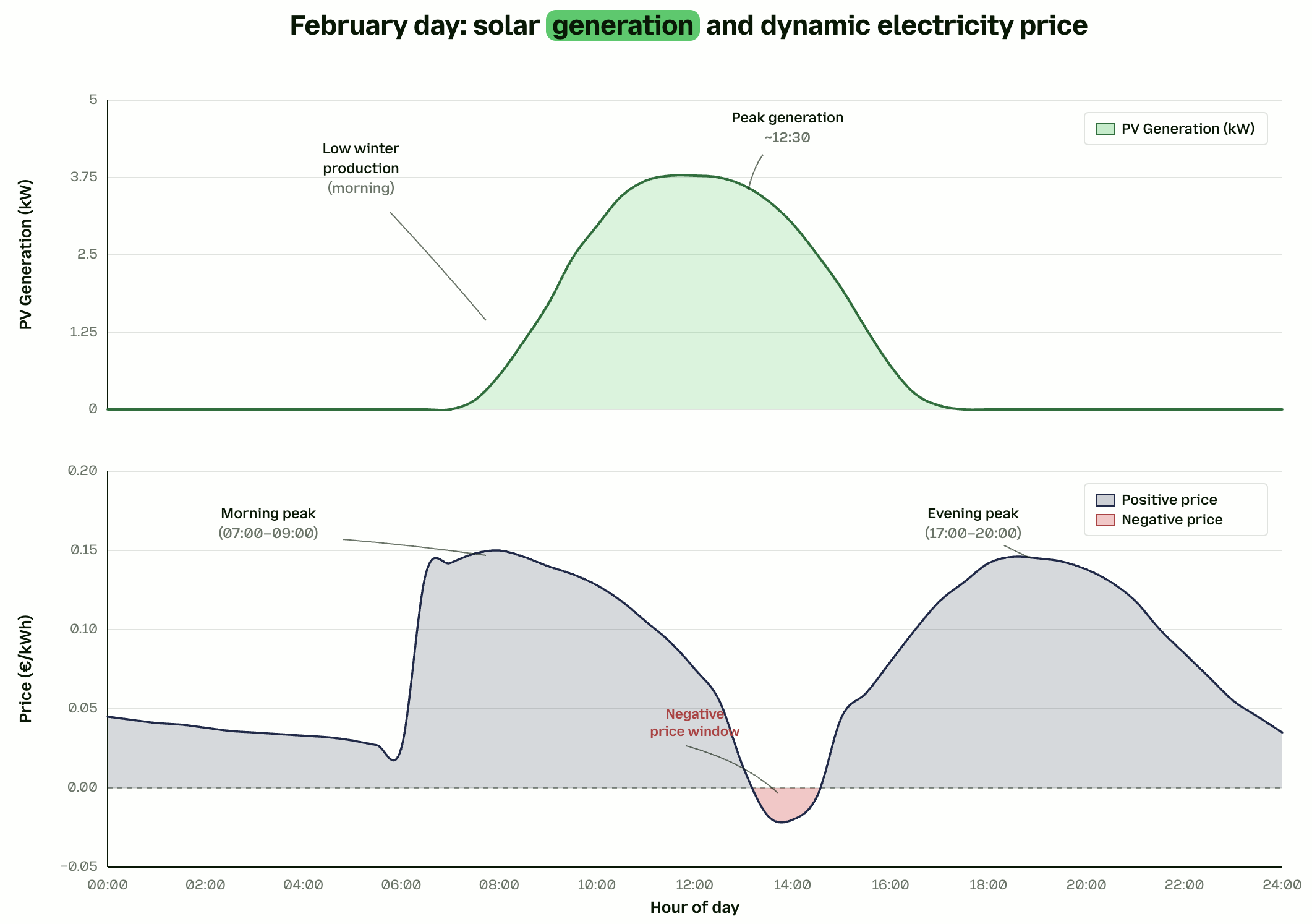
This is where machine learning earns its place. Weather providers like ECMWF give us irradiance, cloud cover and temperature, but they say nothing about how a particular array, with its orientation, tilt, shading and degradation, will turn that weather into kilowatt hours. The ML layer learns that mapping per asset, and learns its quirks: this rooftop systematically underperforms on overcast mornings by a predictable margin.

The same logic applies to load. A model trained on consumption history learns that Tuesday evenings in February look different from Saturday mornings in August, and that this household reliably spikes at 07:30 when the heat pump kicks in. Forecasting is simply supervised learning on time series data, constrained by physics, and continuously retrained as more observations arrive.

Data engineering and MLOps

Each household has its own model, and its parameters drift as winter turns into spring. Retraining has to happen on a regular cadence, per asset. Inference happens far more often: every time a new weather forecast arrives, every PV forecast in the portfolio needs refreshing within minutes. None of it is glamorous, all of it is essential, and getting it wrong is the difference between a portfolio that responds to reality and one running on yesterday's assumptions.

Optimisation: choosing when to charge and discharge

Given those forecasts, the optimiser solves a decision problem over a rolling horizon. The objective is the schedule that minimises the energy bill, or maximises margin, or minimises carbon. The constraints are battery physics, grid connection limits, customer comfort rules and any committed flexibility obligations.

A mixed-integer linear programme (MILP) is the optimisation solved in a single run. Model predictive control (MPC) is the loop around it: as new measurements and forecasts arrive, it re-runs the optimisation, takes the next action, then forecasts, plans and steers again. The MILP is the maths of a single decision; MPC is the discipline of continuously redeciding as reality unfolds.

Dispatching the plan

We rarely have direct, high-frequency control over residential and smaller C&I hardware. Instead we talk to inverter and battery cloud APIs, which expose a limited set of modes: charge, discharge, self consumption, zero feed-in, idle. The continuous power values from the solver have to be translated into a sequence of discrete modes, so the asset behaves, in aggregate, as close as possible to what the optimiser asked for.

A day in the life of the optimiser

It is a March Sunday. Locally it is partly cloudy, so this roof will not fill the battery on its own. Across the wider system, solar is high enough to push day ahead prices negative around midday.

• 09:00 to 13:00: charge the battery, but don't feed into the grid because prices are negative.
• 13:00 to 14:00: top up the battery from the grid alongside the solar to take advantage of negative prices.
• 14:00 to 07:00: use the stored energy to cover the household's load.
• 07:00 to 09:00: the grid needs extra energy, so the battery discharges as a flex activation, and the household is paid for providing it.
• 09:00 to 10:00: feed the solar into the grid, because right now the export reward is higher than at midday.

From single asset to portfolio and grid

When you aggregate thousands of PV-battery systems, the logic does not simply run in parallel. A cluster of batteries all discharging into the same low voltage feeder at 18:00 can cause voltage rise and congestion. A good portfolio optimiser coordinates dispatch across the portfolio to stay within grid constraints.

That creates an opportunity. A well coordinated portfolio of home batteries is, from the grid's perspective, a controllable, dispatchable asset. DSOs can call on it to relieve congestion, balance responsible parties can use it to reduce imbalance, and TSOs can activate it for frequency containment.

In practice the coordination layer combines three streams at once: the physical state of every asset, the live picture of the local grid, and the live picture of the markets. For each interval the platform decides which assets are best placed to respond, and to which signal. For IPPs running large BESS and PV plants the problem is identical in structure; we see this with DSG in the Netherlands, routing flexibility across intraday, day ahead and congestion markets.

What good optimisation looks like

• Charging follows prices, not the clock. A battery that always charges at the same time is running a fixed schedule, not an optimiser.
• The battery is rarely full before the PV peak. A good optimiser preserves headroom for solar.
• Back-feeding is managed, not maximised. Where injection is constrained or penalised, excess PV is held or absorbed.
• Intraday corrections are visible. A system with real-time feedback adjusts when forecasts are wrong.

Reading a chart after the fact and answering why a mode was chosen is genuinely hard, even for engineers. It is also a support problem in disguise: every decision an end customer cannot make sense of is a potential ticket. Clear explanations of optimiser decisions are as much a product requirement as the optimiser itself.

The role of engineers and software

The models, the objective function and the constraints are the engineering work. Execution and scaling are the software problem: running it continuously across thousands of assets, with reliable connectivity to meters, inverters and market APIs, and the observability to know when something has gone wrong.

Powernaut brings both sides together, from single residential systems through aggregated portfolios to large scale BESS and PV plants. If you are building or aggregating PV-battery portfolios at any scale, the team is happy to walk through the specifics.